

Certain stocks exhibit consistent trends, while others don't. Despite drops, some companies' stock prices rebound. The common solution for both scenarios is time series models.
According to a recent study by the University of California, Berkeley, Autoregressive models are one of the most commonly used methods for time series forecasting.
The values of past and present time series frequently overlap. As a result, such data exhibit autocorrelation. As a result, knowing a product's current pricing allows us to anticipate its valuation tomorrow roughly.
So, in this article, we will explain the autoregressive model that captures this correlation.
Understanding Time Series Data
Understanding and identifying these different time series patterns is crucial for choosing appropriate modeling techniques and accurately forecasting future values. It allows analysts to apply specific methods tailored to the patterns observed in the data, improving the accuracy of time series forecasting models.
Definition of Time Series Data
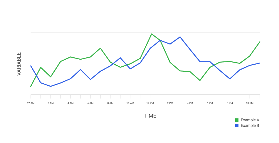
Time series data refers to a sequence of data points collected over time, where the values are recorded at regular intervals. It represents the evolution of a variable or phenomenon over a specific period. The data points are typically indexed by the time of collection, allowing for analysis of trends, patterns, and dependencies within the data.
Time series data can be univariate, consisting of a single variable recorded over time, or multivariate, where multiple variables are observed simultaneously. Examples of time series data include stock prices, temperature readings, sales figures, and economic indicators.
Types of Time Series Patterns
Time series data often exhibit specific patterns that can be categorized into different types:
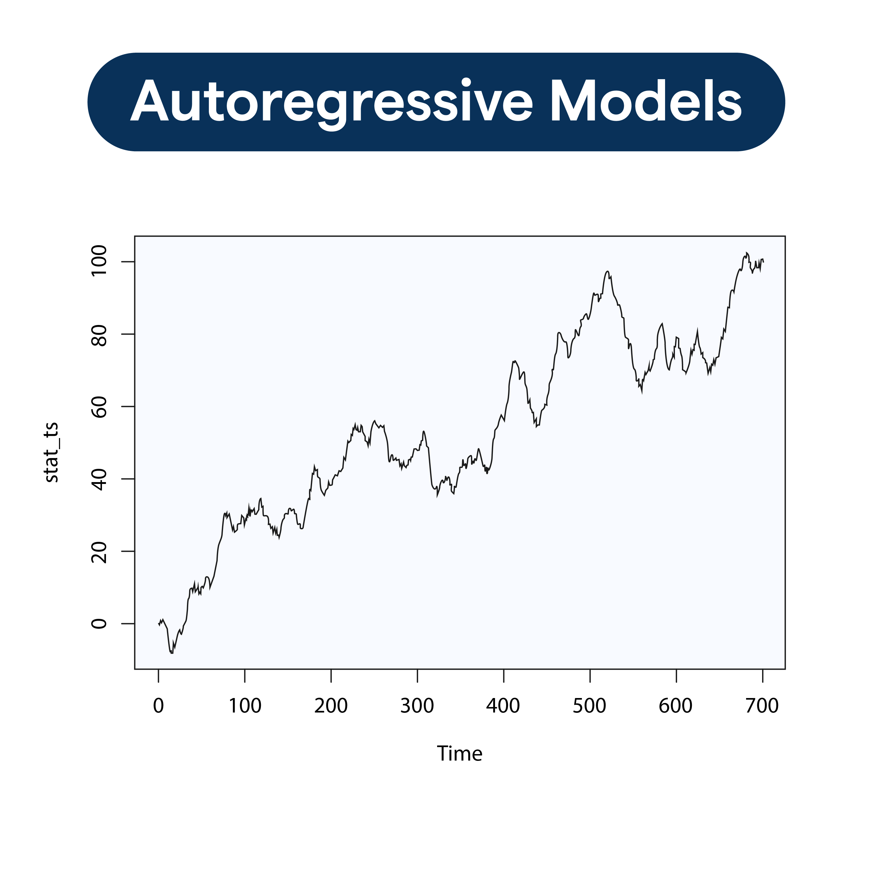
- Trend: Trend refers to the long-term movement or directionality of the data. It represents the underlying growth or decline in the variable over time. Trends can be upward (increasing), downward (decreasing), or stable.
- Seasonality: Seasonality refers to a regular pattern that repeats within fixed and known time intervals. It occurs when data exhibits systematic variations linked to specific seasons, months, weeks, or days of the week. Seasonal patterns often result from natural factors like weather, holidays, or business cycles.
- Cyclical Variations: Cyclical variations represent irregular patterns that occur over some time longer than a year. They are often associated with economic fluctuations, such as business cycles, investment cycles, or political events. Unlike seasonality, cyclical variations do not have fixed or predictable intervals.
- Irregular or Random Fluctuations: Irregular or random fluctuations, also known as noise, represent unpredictable and unexplained variations in the data. They can result from random events, measurement errors, or unpredictable factors that impact the variable.
Basics of Autoregressive Models
The order of autoregressive models denoted as p, represents the number of lagged values used to predict the current value. Selecting the appropriate order is crucial in autoregressive modeling.
A higher order (more significant p) allows for capturing complex dependencies but may increase model complexity and risk overfitting.
Conversely, a lower order may oversimplify the model and fail to capture essential dynamics in the data.
Definition and Components of Autoregressive Models
Autoregressive models are statistical models used to predict future values of a variable based on its past values.
The term "autoregressive" implies that the current value of the variable is regressed on its lagged (past) values.
The primary components of autoregressive models are the current value of the variable (dependent variable) and one or more of its lagged values (independent variables).
Autocorrelation and the Concept of Lag
Autocorrelation refers to the correlation between a variable and its lagged values. It measures the degree of relationship between observations at different time points. Autocorrelation at lag k, denoted as AC(k), quantifies the linear association between a variable at time t and its value at time t-k.
Lag refers to the time gap between the current observation and its lagged value. In autoregressive models, the choice of lag is crucial as it determines the number of past values used in predicting the current value. Lag k indicates that k previous observations are considered in the model.
Stationarity and its importance in Autoregressive Models
Stationarity is a fundamental property of time series data important for autoregressive modeling. A stationary time series exhibits constant statistical properties, such as constant mean, variance, and autocovariance structure.
Stationarity is crucial in autoregressive models because it ensures that the relationship between the current value and its lagged values remains stable.
When dealing with non-stationary data, the estimation and interpretation of autoregressive models can be challenging.
Therefore, it is often necessary to transform or manipulate non-stationary data to achieve stationarity before applying autoregressive modeling techniques.
Common techniques for achieving stationarity include differencing, logarithmic transforms, or seasonal adjustments.
Order of Autoregressive Models
Choosing the optimal order often involves statistical techniques like the Akaike Information Criterion (AIC) or Bayesian Information Criterion (BIC), which aim to balance model fit and complexity. Iterative approaches, such as autocorrelation and partial autocorrelation plots, can also help determine the order by examining the significant lags and cutoff points.
Understanding the concept of order is essential for building effective autoregressive models, as it influences model accuracy and interpretability.
Building Autoregressive Models
Before building autoregressive models, it is essential to prepare the data and perform exploratory analysis.
Data Preparation and Exploratory Analysis
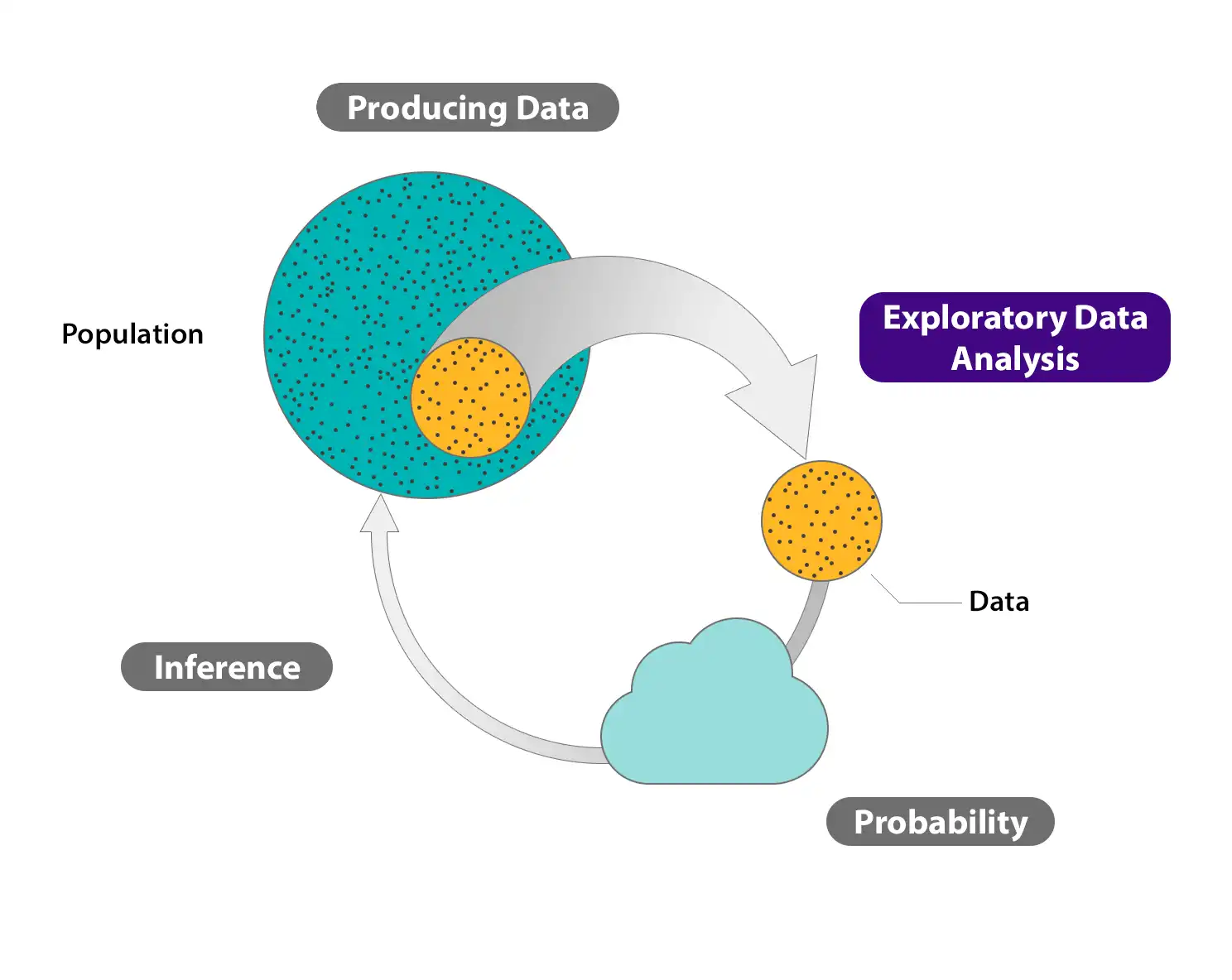
Data preparation involves cleaning, transforming, and organizing the time series data in a format suitable for modeling. This may include handling missing values, smoothing noisy data, standardizing variables, and addressing non-stationarity issues.
Exploratory analysis aims to gain insights into the characteristics of the time series data.
It involves visualizing the data using lines, scatter, histograms, or box plots to identify trends, seasonality, outliers, or other patterns.
Exploratory analysis also helps in understanding the level of autocorrelation and determining the appropriate order for the autoregressive model.
Determining the order of the Autoregressive Model
The order of the autoregressive model, denoted as p, determines the number of lagged values used to predict the current value. Determining the order is crucial, as an inappropriate choice can lead to poor model performance. There are several approaches to determine the order, including:
- Autocorrelation Function (ACF) and Partial Autocorrelation Function (PACF): ACF and PACF plots can help identify significant lags and their cutoff points, indicating the appropriate order for the autoregressive model.
- Information criteria (e.g., AIC, BIC): These statistical criteria balance model fit and complexity. They can be used to compare different models with varying orders and select the optimal order that minimizes the information criterion.
- Iterative approaches: By evaluating the performance of autoregressive models with different orders, one can observe the model's behavior with varying lags. This iterative process can help determine the most suitable order for the autoregressive model.
Estimating Model Coefficients using Various Methods
Once the order is determined, estimating the model coefficients is next. There are various methods for estimating the coefficients in autoregressive models, including:
- Ordinary Least Squares (OLS): This method estimates the coefficients by minimizing the sum of squared differences between the predicted and actual values. OLS assumes that the error terms are normally distributed and have constant variance.
- Yule-Walker equations: These equations provide a method to estimate the autoregressive coefficients directly from the autocovariance function.
- Maximum Likelihood Estimation (MLE): MLE estimates the coefficients by maximizing the likelihood function, which measures how likely the observed data is under the proposed autoregressive model.
If you are the one who likes the no coding chatbot building process, then meet BotPenguin, the home of chatbot solutions. With all the heavy work of chatbot development already done for you, simply use its drag-and-drop feature to build an AI-powered chatbot for platforms like:
- WhatsApp Chatbot
- Facebook Chatbot
- Wordpress Chatbot
- Telegram Chatbot
- Website Chatbot
- Squarespace Chatbot
- Woocommerce Chatbot
Assessing Model Performance and Accuracy Metrics
After estimating the model coefficients, assessing the model's performance and evaluating its accuracy is essential. This involves using appropriate metrics to measure how well the autoregressive model fits the data and predicts future values. Common accuracy metrics for time series models include:
- Mean Absolute Error (MAE): This metric measures the average absolute difference between the predicted and actual values.
- Root Mean Squared Error (RMSE): RMSE is the square root of the average squared difference between the predicted and actual values. It penalizes more significant errors more heavily than MAE.
- Mean Absolute Percentage Error (MAPE): MAPE calculates the average percentage difference between the predicted and actual values, providing a measure of relative error.
Other metrics such as R-squared, Akaike Information Criterion (AIC), or Bayesian Information Criterion (BIC) can also provide insights into the model's goodness of fit and allow for model comparison.
Time Series Forecasting with Autoregressive Models
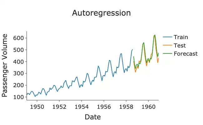
Autoregressive models can be utilized for forecasting future values of a time series variable based on its past values. Once an autoregressive model is built and its coefficients are estimated, it can generate predictions for future time points.
Using Autoregressive Models for Future Predictions
By using previous values of the variable, the model can capture the inherent patterns and dependencies in the data, allowing for reasonably accurate predictions.
The autoregressive model can be recursively applied to make future predictions by using the predicted values as inputs for the subsequent time points. For example, if an AR(p) model is built, the model equation can forecast the value at time t+1 by substituting the lagged values up to t with the corresponding predicted values.
Evaluating Forecast Accuracy and Dealing with Model Limitations
After generating forecasts with the autoregressive model, assessing the predictions' accuracy and understanding the model's limitations is crucial. Several techniques can be employed to evaluate the forecast accuracy:
- Backtesting: Backtesting evaluates a model by comparing its predictions with actual values from a separate, unused period to assess generalization to unseen data.
- Accuracy metrics: Accuracy metrics, like MAE or RMSE, quantify differences between predicted and actual values, providing insights into a model's precision and enabling method comparisons.
- Residual analysis: Residual analysis identifies patterns or missed variables in a model by examining its errors.
Advanced Techniques and Considerations in Autoregressive Modeling
While autoregressive models provide a solid foundation for time series forecasting, some advanced techniques and considerations can enhance their performance:
- Seasonality: Autoregressive models typically assume the absence of seasonality. If the time series exhibits seasonal patterns, including seasonal terms in the model, such as SARIMA or Fourier terms, it may be beneficial to capture these variations.
- Exogenous variables: Autoregressive models can be extended to include exogenous variables, which are external variables that may influence the time series. Incorporating relevant exogenous variables can improve forecast accuracy by accounting for additional factors that impact the target variable.
- Model selection and combination: Instead of relying solely on autoregressive models, it can be beneficial to explore other forecasting techniques, such as moving average models, exponential smoothing, or machine learning algorithms. Model selection and combination approaches, like model averaging or ensemble methods, can help leverage the strengths of multiple models and improve forecast accuracy.
- Online learning: Autoregressive models can be adapted to handle streaming data or real-time forecasting scenarios using online learning techniques. Online learning allows the model to update and incorporate new observations as they become available, ensuring that the forecasting remains up-to-date.
Conclusion
The autoregressive model forecasts the future based on past data. Technical analysts widely use them to forecast future security prices. Time series values are associated with their predecessors and successors in this analysis.
Autoregressive models use the squared coefficient of previous values to predict the next value in a vector time series.
Autoregressive models are statistical models that have proven effective for us in various applications, including time series and financial forecasting. They are also used to build models from time series data.
Frequently Asked Questions (FAQs)
What is an autoregressive model, and how does it work?
An autoregressive model is used for time series forecasting. It relies on the relationship between past values of the variable and its current value to make predictions for the future.
How do I determine the order of an autoregressive model?
The order of an autoregressive model determines the number of lagged values used for prediction. It can be determined using autocorrelation, partial autocorrelation functions, or information criteria.
What are some common techniques for estimating autoregressive model coefficients?
Some common techniques for estimating autoregressive model coefficients include ordinary least squares, Yule-Walker equations, and maximum likelihood estimation. These methods determine the relationship between current and past values of the time series.
How do I evaluate the accuracy of autoregressive model forecasts?
The accuracy of autoregressive model forecasts can be evaluated using metrics such as mean absolute error, root mean squared error, and mean absolute percentage error. Backtesting and analyzing residuals can also provide insights into model performance.
Can autoregressive models handle time series data with seasonality?
Autoregressive models typically assume the absence of seasonality. However, extensions like SARIMA or Fourier terms can be included to capture seasonal patterns and improve forecast accuracy.
Are there any advanced techniques to enhance autoregressive model forecasting?
Yes, there are advanced techniques to enhance autoregressive model forecasting. These include incorporating exogenous variables that may influence the time series, model selection and combination approaches, and online learning techniques for real-time forecasting.